This module is used to calculate the difficulty of a decision based on a set of forecasts,
such as an ensemble, for quantities such as wind speed or significant wave height as a
function of space and time.
where \(\sigma\) is the ensemble standard deviation, \(\bar{x}\) is the ensemble mean,
\(P(x_{i,j}\geq thresh)\) is the ensemble (sample) probability of being greater than or equal
to the threshold, and \(P(x_{i,j}<thresh)\) is the ensemble probability of being less than
the threshold. The \((\sigma/\bar{x})\) expression is a measure of spread normalized by the
mean, and it allows one to identify situations of truly significant uncertainty. Because the
difficulty index is defined only for positive definite quantities such as wind speed or significant
wave height, division by zero is avoided. \((\sigma/\bar{x})_{ref}\) is a (scalar) reference
value, for example the maximum value of \((\sigma/\bar{x})\) obtained over the last 5 days as
a function of geographic region.
The first term in the outer brackets is large when the uncertainty in the current forecast is
large relative to a reference. The second term is minimum when all the probability is either
above or below the threshold, and maximum when the probability is evenly distributed about the
threshold. Therefore, it penalizes the split case, where the ensemble members are close to evenly
split on either side of the threshold. The A term outside the brackets is a weighting to account
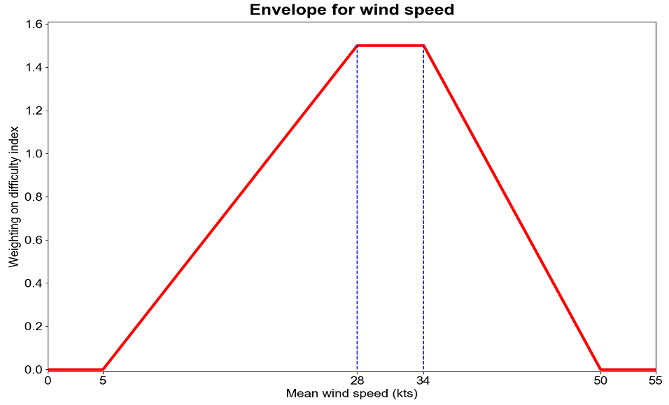
for heuristic forecast difficulty situations. Its values for winds are given below.
A = 0 if \(\bar{x}\) is above 50kt
A = 0 if \(\bar{x}\) is below 5kt
A = 1.5 if \(\bar{x}\) is between 28kt and 34kt
A = \(1.5 - 1.5[\frac{\bar{x}(kt)-34kt}{16kt}]\) for 34kt \(\leq\bar{x}\leq\) 50kt
A = \(1.5[\frac{\bar{x}(kt)-5kt}{23kt}]\) for 5kt \(\leq\bar{x}\leq\) 28kt
Figure 3.1 Weighting applied to wind difficulty index.
The weighting ramps up to a value 1.5 for a value of x that is slightly below the threshold.
This accounts for the notion that a forecast is more difficult when it is slightly below the threshold
than slightly above. The value of A then ramps down to zero for large values of
\(\bar{x}_{i,j}\).
To gain a sense of how the difficulty index performs, consider the interplay between probability of
exceedance, normalized ensemble spread, and the mean forecast value (which sets the value of
A) shown in Tables 3.1-3.3. Each row is for a different probability of threshold exceedance,
\(P(x_{i,j} \geq thresh)\), each column is for a different value of normalized uncertainty,
quantized as small, \((\sigma/\bar{x})/(\sigma/\bar{x})_{ref}=0.01\), medium,
\((\sigma/\bar{x})/(\sigma/\bar{x})_{ref}=0.05\), and large,
\((\sigma/\bar{x})/(\sigma/\bar{x})_{ref}=1.0\). Each box contains the calculation of
\(d_{i,j}\) for that case.
When \(\bar{x}\) is very large or very small the difficulty index is dominated by A.
Regardless of the spread or the probability of exceedance the difficulty index takes on a value near
zero and the forecast is considered to be easy (Table 3.1).
When \(\bar{x}\) is near the threshold (e.g. 25kt or 37kt), the situation is a bit more complex
(Table 3.2). For small values of spread the only interesting case is when the probability is
equally distributed about the threshold. For large spread, all probability values deserve a look, and
the case where the probability is equally distributed about the threshold is deemed difficult.
When \(\bar{x}\) is close to but slightly below the threshold (e.g. between 28kt and 34kt),
almost all combinations of probability of exceedance and spread deserve a look, and all values of the
difficulty index for medium and large spread are difficult or nearly difficult (Table 3.3).
Table 3.1 Example of an easy forecast where \(\bar{x}\) is very large (e.g. 48 kt) or very small (e.g. 7kt), making \(A/2=0.1/2=0.05\).
Prob of Thresh Exceedance
Small Spread
Medium Spread
Large Spread
1
0.05*(0.01+0.5) = 0.026
0.05*(0.5+0.5) = 0.05
0.05*(1+0.5) = 0.075
0.75
0.05*(0.01+0.75) = 0.038
0.05*(0.5+0.75) = 0.063
0.05*(1+0.75) = 0.088
0.5
0.05*(0.01+1) = 0.051
0.05*(0.5+1) = 0.075
0.05*(1+1) = 0.1
0.25
0.05*(0.01+0.75) = 0.038
0.05*(0.5+0.75) = 0.063
0.05*(1+0.75) = 0.088
0
0.05*(0.01+0.5) = 0.026
0.05*(0.5+0.5) = 0.05
0.05*(1+0.5) = 0.075
Table 3.2 Example of a forecast that could be difficult if the conditions are right, where \(\bar{x}\) is moderately close to the threshold (e.g. 25kt or 37kt), making \(A/2=1/2=0.5\).
Prob of Thresh Exceedance
Small Spread
Medium Spread
Large Spread
1
0.5*(0.01+0.5) = 0.26
0.5*(0.5+0.5) = 0.5
0.5*(1+0.5) = 0.75
0.75
0.5*(0.01+0.75) = 0.38
0.5*(0.5+0.75) = 0.63
0.5*(1+0.75) = 0.88
0.5
0.5*(0.01+1) = 0.51
0.5*(0.5+1) = 0.75
0.5*(1+1) = 1.0
0.25
0.5*(0.01+0.75) = 0.38
0.5*(0.5+0.75) = 0.63
0.5*(1+0.75) = 0.88
0
0.5*(0.01+0.5) = 0.26
0.5*(0.5+0.5) = 0.5
0.5*(1+0.5) = 0.75
Table 3.3 Example of a situation that is almost always difficult, where \(\bar{x}\) is at or slightly below the threshold (e.g. 28kt to 34kt), making \(A/2=1.5/2=0.75\).